Pipeline description
BabelBrain takes 3D imaging data (MRI and, if available, CT) along with a trajectory indicating the location and orientation of an ultrasound transducer to target a location in the brain.

Currently, 17 types of transducers are supported:
| Device model | Type | Frequency/ies (kHz) | # Elements | Focusing length (mm) | Diameter (mm) |
|---|---|---|---|---|---|
| Single | Single element shell | User-defined | 1 | User-defined | User-defined |
| BSonix | Set of 4, shell single element | 650 | 1 | 33, 55, 65, 80 | 48, 61, 61, 61 |
| H246 | Flat annular array | 500 | 2 | - | 33.6 |
| CTX_250 | Shell annular array | 250 | 4 | 63.2 | 64.5 |
| CTX_250-2ch | Shell annular array | 250 | 2 | 63.2 | 64.5 |
| CTX_500 | Shell annular array | 500 | 4 | 63.2 | 64.5 |
| DPX_500 | Shell annular array | 500 | 4 | 144.9 | 64 |
| DPXPC_300 | Shell annular array | 300 | 4 | 144.9 | 64 |
| R15287 | Shell annular array | 300 | 10 | 65 | 75 |
| R15473 | Shell annular array | 300 | 10 | 65 | 100 |
| H317 | Shell phased array | 250, 700, 825 | 128 | 135 | 150 |
| I12378 | Shell phased array | 650 | 128 | 72 | 103 |
| R15148 | Shell phased array | 500 | 128 | 80 | 103 |
| ATAC | Shell phased array | 650 | 128 | 72 | 103 |
| R15646 | Shell phased array | 650 | 64 | 65 | 66 |
| IGT64_500 | Shell phased array | 500 | 64 | 75 | 65 |
| REMOPD | Flat phased array | 300, 480, 490 | 256 | - | 58 |
Overall workflow
The typical TUS workflow working with BabelBrain is shown below
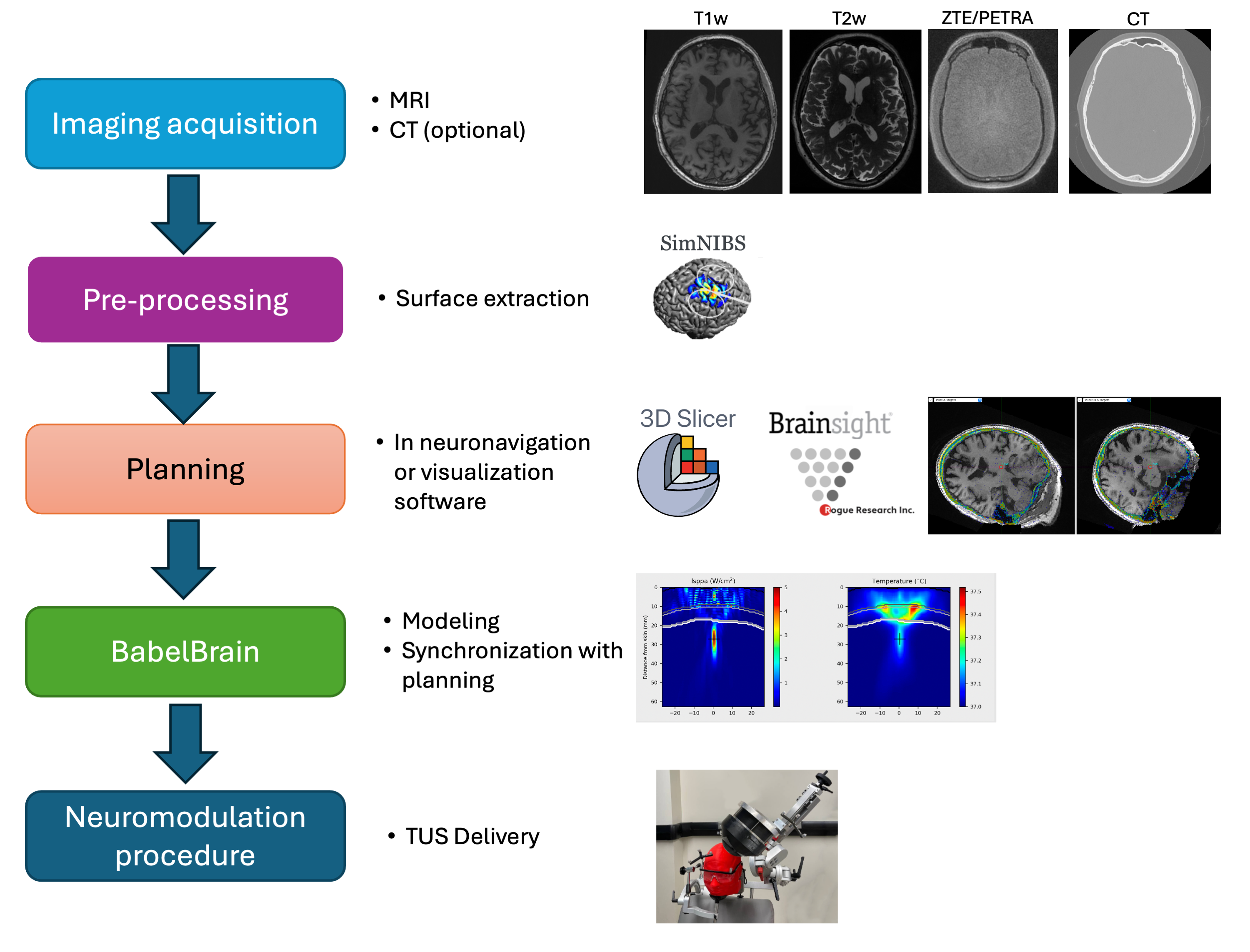
The next sections cover these steps